Tackling batch effects and bias
in transcript expression
Michael Love
@mikelove
EuroBioc2015
December 7, 2015
this talk: http://mikelove.github.io/eurobioc2015
Two parts:
- RNA-seq sequence biases
- Implications for exon, transcript, and gene differential analysis
Some RNA-seq biases
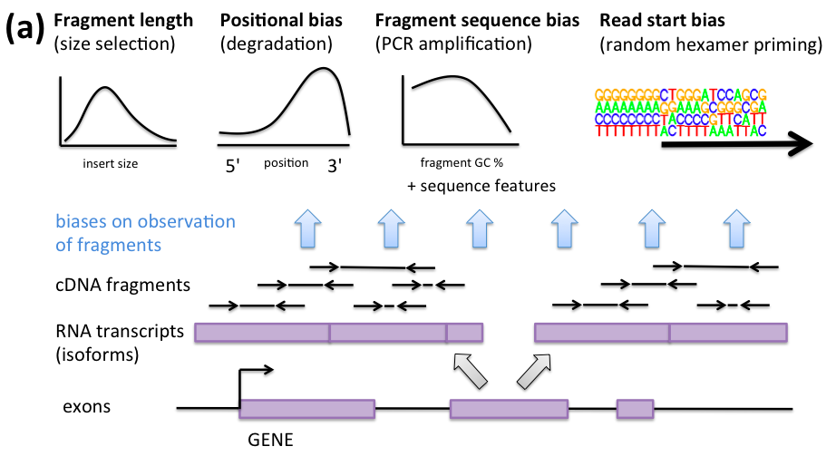
Sequence bias correction

- A great paper on concepts of RNA-seq bias and correction
- Random hexamer priming is most important. Used by Cufflinks, eXpress, BitSeq, kallisto.
- GC content of transcript doesn't capture the bias
- "although normalization of expression values by GC content may be a simple way to remove some bias, it may well be a proxy for other effects rather than of inherent significance"
Does this do the trick?
- 15 vs 15 GEUVADIS samples across sequencing center
- Cufflinks with random hexamer bias correction
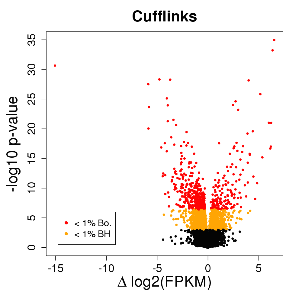
- At 1% FDR, 2,500 transcripts DE (10%)
- 600 genes change major isoform (9%)
- NB: this is a lot of changes!
What's going on?
- Look at genes with 2 isoforms and reporting DE
- Find the critical regions exclusive to one or other isoform
- Calculate GC content of those regions

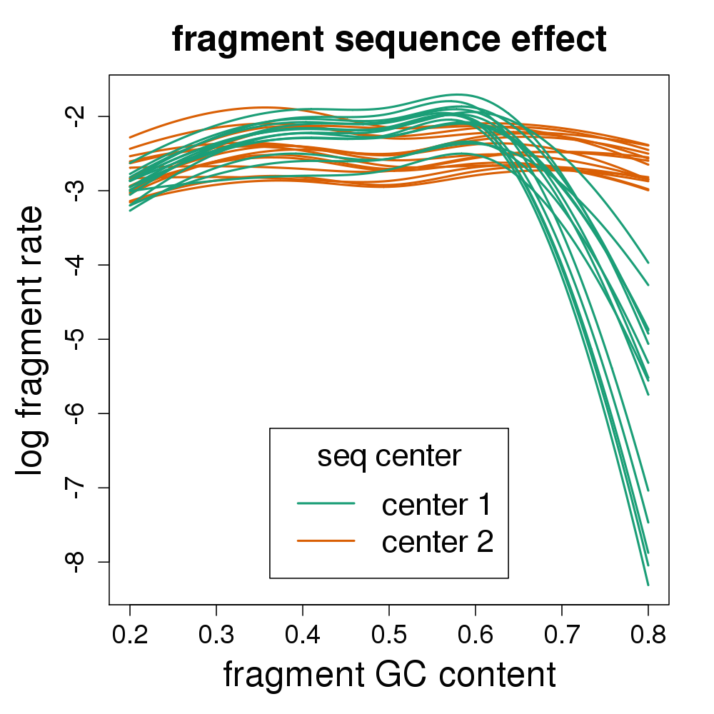
Idea:
- Inspiration from Benjamini and Speed, 2012
- The correct resolution for GC content bias is at the fragment level, the unit which is PCR amplified
- Include in the RNA-seq model the probability of observing a fragment, given its GC content
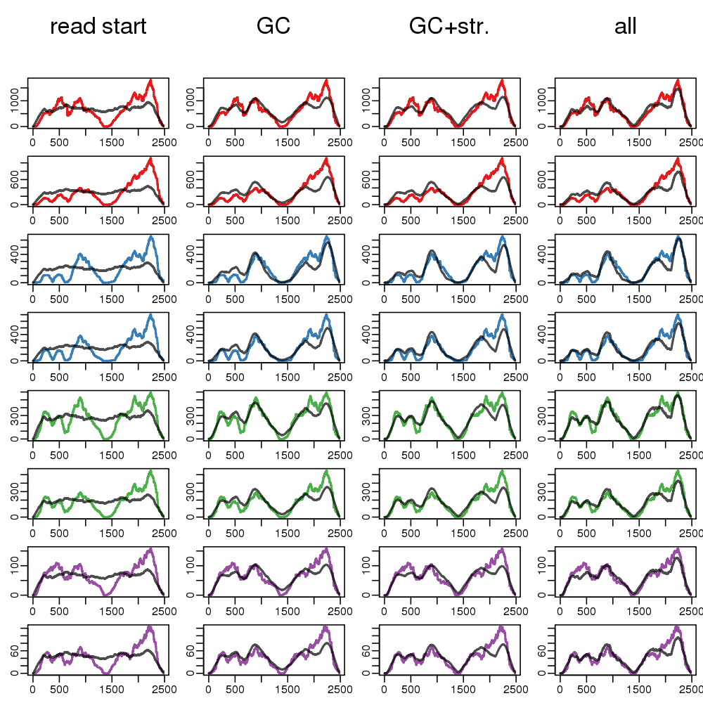
A dataset where we know the exact sequence
- Lahens et al (2014): IVT-seq
- Predict coverage along the troublesome transcripts using:
- read start bias (Cufflinks VLMM)
- fragment GC content (+ long stretches G|C)

- color = coverage; black = test set prediction
- more examples in supplementary slides and ms
Systematic comparison
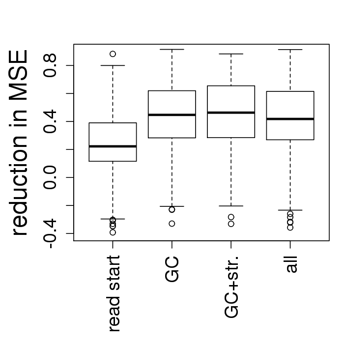
- Fragment GC explains 2x more coverage variability
- Adding read start to the fragment GC: no improvement
alpine: a transcript quant method for comparing bias models
- read start bias (Cufflinks VLMM)
- fragment length
- positional bias
- fragment GC content
Back to 15 vs 15 GEUVADIS samples across sequencing center
Four fold reduction in false positives
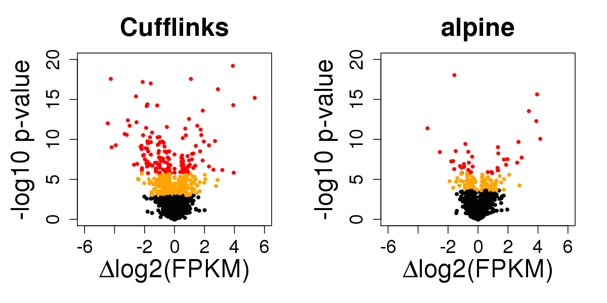
- 562 ⇒ 136 at FDR 1%
- alpine controls sensitivity in simulation (supp. slides)
- What are these Cufflinks false positives from?
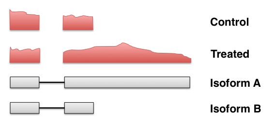
Coverage drop-out from fragment GC
- No existing quantification method corrects for this bias
- There are many genes with critical regions in this range
- Other experiments have problems with low GC
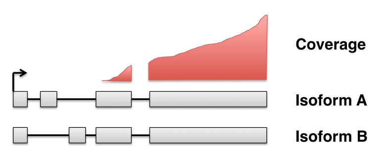
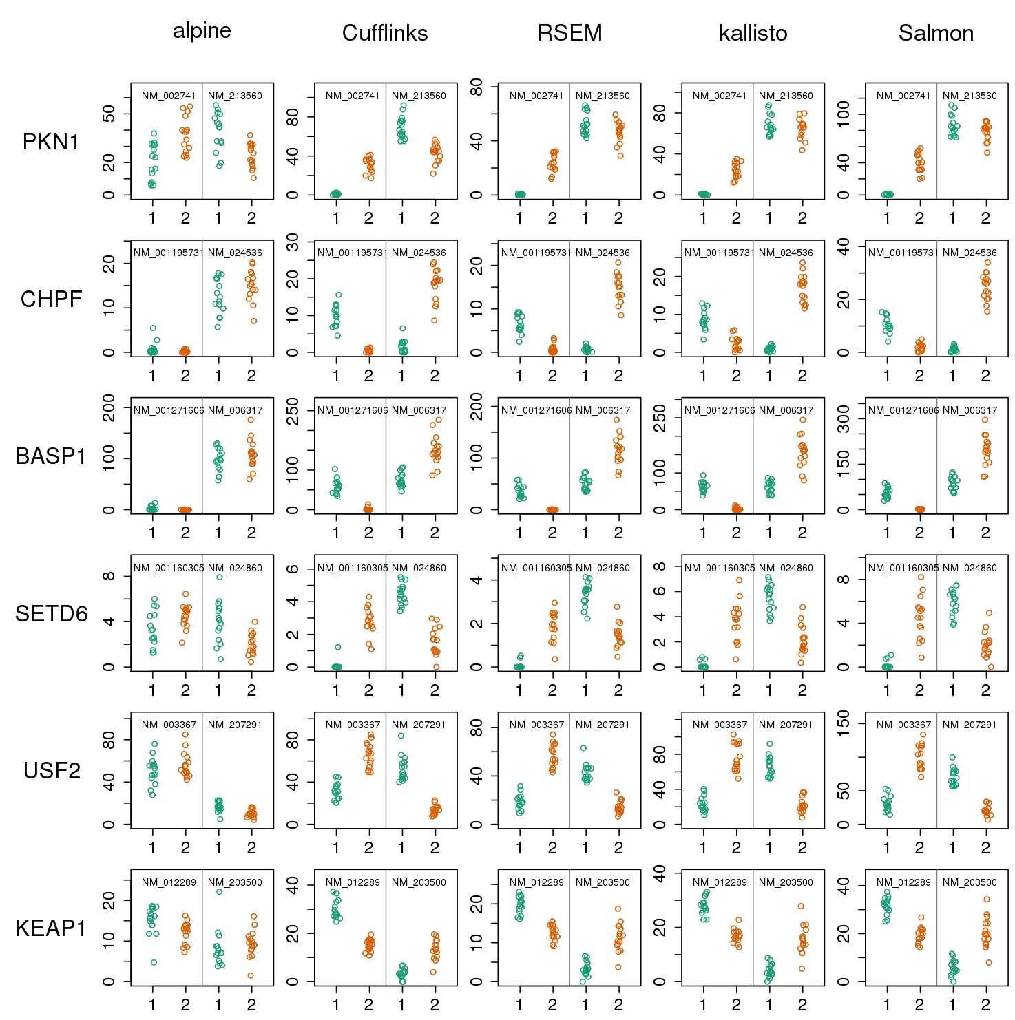
Misidentified isoforms from coverage variability
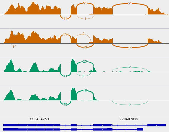
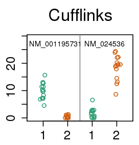
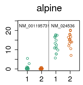
- Regardless of junction spanning evidence, naive quant methods are tricked by variable coverage
- What about k-mer / pseudo-alignment methods?
Pseudo-alignment: same misidentified isoforms
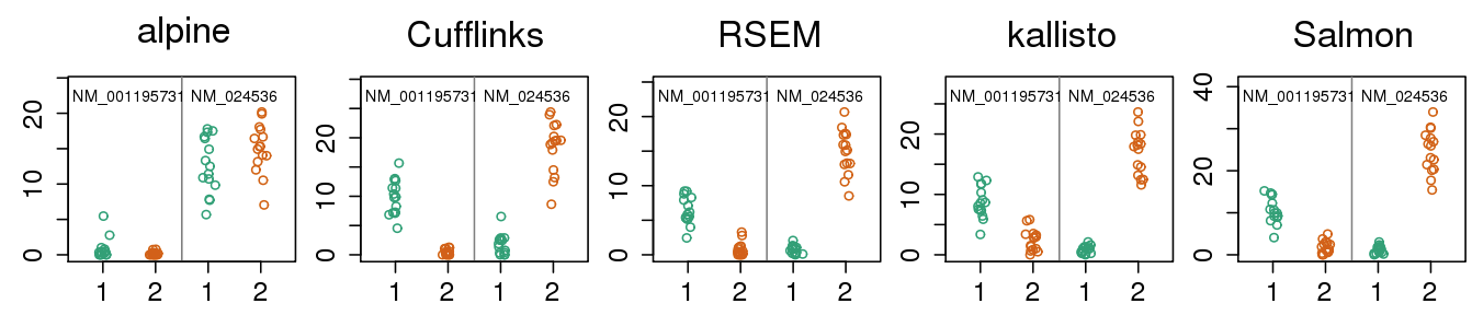
- Missing k-mers cause same problem as missing fragments for a model which does not expect coverage drop-out
- More examples in supp slides
- Out of 5,700 tx: 136, 562, 577, 548, 614 false positives of DE
Summary part 1
- No existing quant methods correct for fragment GC content
- Not just a batch problem, we see ~10% wrongly identified transcripts in the samples with coverage variability
- Lahens et al (2014): bias may occur due to underlying biology
- Simulations often do not include coverage variability, so not learning much about accuracy for real data
- See manuscript for more details, examples: alpine ms
Implications for differential analysis
- Exon usage corrected using exon GC content as covariate
- Exon usage corrected by balanced design and blocking factor
- Transcript-level perfect coverage: OK
- Transcript-level confounded: many FP
- Transcript-level balanced could attribute DE to wrong isoform
- Gene-level reduces problem of misidentified isoforms
Gene-level count criticisms
- Counts are correlated with feature length: Trapnell et al (2013)
- Discarding multi-mapping fragments can lead to false negatives: Robert & Watson (2015)
- Gene-level "masks" differential tx usage
Gene-level count defenses
- Differential tx usage doesn't necessarily lead to large bias
- Among multi-isoform genes, most tx are similar length: median difference of ~15%
- Gene-level and sub-gene-level are complementary
- Transcript estimation is sometimes unidentifiable
Why still counts?
- While TPM good for descriptive measure
- Statisticians want: counts & offset/exposure
- (Library size is an offset)
- I counted 10 penguins in 1 hr and 20 penguins in 2 hrs
- (Mostly important when sample size is small-ish)
New quantification methods
- Sailfish/Salmon and kallisto are game changing methods
- Quantification from FASTA in minutes
- For those who still want gene-level DE
… and to reduce problems of bias and unidentifiability:- Summarize counts (or estimated counts) to gene-level
- Calculate offset based on average transcript length
- Then do complementary exon- or tx-level analysis
Importing for count-based methods
- Charlotte Soneson and Mark Robinson have extensively studied using these quant methods + Bioconductor pkgs, manuscript in preparation
- Together, worked on a package, tximport: import counts and offset (+ other options)
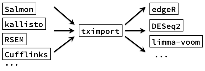
- (RSEM always provided average transcript length)
- (not using bootstrap variances)
Acknowledgments
- Rafael Irizarry
- John Hogenesch at UPenn for IVT-seq dataset
- Bioc core team:
alpinedepends on e.g.findCompatibleOverlaps - Supported by NIH cancer training grant
- Charlotte Soneson and Mark Robinson on
tximportcollaboration
Supplementary slides
More examples of IVT-seq coverage
Isoform misidentification in GEUVADIS
alpine sensitivity in simulation

- simulated confounding with GC bias from GEUVADIS
alpine accuracy in simulation
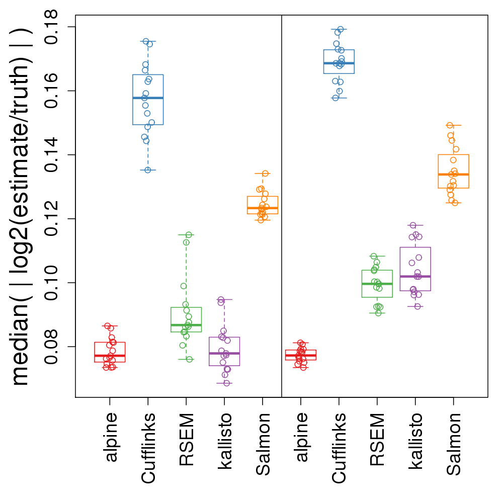
- median absolute error for abundance
- left: less GC bias; right: more GC bias
software details
- alpine 0.1.1 with GC content and fragment length
- Cufflinks 2.2.1 with bias correction
- RSEM 1.2.11
- kallisto 0.42.3 with bias correction
- Salmon 0.5.0 without bias correction (better performance)